
|
|
COS 429 - Computer Vision |
Fall 2016 |
| Course home | Outline and Lecture Notes | Assignments |
Binary classifiers: Your first task is to implement a learning method called logistic regression, for performing binary classification. In this method, you have a training set consisting of a number of data points $x_i$, each of which is a feature vector, and a class label $z_i \in \{0,1\}$ for each. (Note that in class we used -1 and 1 as the class labels - we will use 0 and 1 for the purposes of this assignment.) Your job is to learn a model that will take new data points and predict the class for each one.
Linear regression is the simplest way of finding a classifier.
You just set up a set of linear equations
$$
z_1 = a + b x_{11} + c x_{12} + d x_{13} + \ldots
$$
$$
z_2 = a + b x_{21} + c x_{22} + d x_{23} + \ldots
$$
and least-squares solve for the parameters $a,b,c,d,$ etc. In the above
equations, the first subscript of $x$ refers to the datapoint, while the
second subscript indexes over the dimensions of $x$.
To use the results of the above linear regression to predict the class for
a new datapoint $y$, you just compute
$$
a + b y_1 + c y_2 + d y_3 + \ldots
$$
and see whether the result is closer to 0 or 1 -
i.e., apply a threshold of 0.5.
How do you do the least-squares solve? Let's first set this up as a matrix equation: $$ X\,\theta = z $$ where $$ X = \begin{pmatrix} 1 & x_{11} & x_{12} & x_{13} & \cdots \\ 1 & x_{21} & x_{22} & x_{23} & \cdots \\ 1 & \vdots & \vdots & \vdots & \ddots \\ \end{pmatrix} , \quad \theta = \begin{pmatrix} a \\ b \\ c \\ d \\ \vdots \end{pmatrix} , \quad \mathrm{and} \quad z = \begin{pmatrix} z_1 \\ z_2 \\ \vdots \end{pmatrix} . $$
Now, we recognize this as an overconstrained linear system, and solve the "normal equations": $$ X^TX\,\theta = X^Tz $$ In Matlab, solving this is as easy as writing
params = (X' * X) \ (X' * z);
(It's also equivalent to params = X \ z; but this is a shortcut we won't be able to use once we look at fancier formulations.)
Regularization:
In our case, the "datapoints" $x_i$ will actually be feature vectors that
we have computed over image patches. In other words, they will be long (have
many dimensions), and might have some redundancies. In this case, there is
a danger that $X^TX$ may be singular or close to singular, especially if we
don't have a lot of training data. In this case, we may regularize the
linear system by encouraging the resulting weights $a,b,c,\ldots$ to lie
close to zero unless there is enough data to pull them away. Mathematically,
this is known as $L_2$ regularization, and works like this:
$$
(X^TX + \lambda\,n\,I)\,\theta = X^Tz
$$
where $I$ is the identity matrix, $n$ is the number of data points, and
$\lambda$ is a small constant, perhaps 0.001. Notice that the matrix
$X^TX$ has been pulled to be a bit closer to a diagonal (since we added
a multiple of the identity to it). This makes is better conditioned -
less likely to be singular. The bigger we make $\lambda$, the more diagonally
dominant it becomes, and we get a more stable (but less accurate) solve.
Logistic regression:
The problem with simple linear regression, as we saw in class, is that it
puts too much emphasis on points far away from the decision boundary.
This is because it is trying to minimize a quadratic loss function:
$$
L = \sum_i (z_i - (a + bx_{i1} + cx_{i2} + dx_{i3} + \ldots))^2
$$
Logistic regression, in contrast, uses a generalized linear model,
meaning that the loss function has a nonlinearity applied to a linear
combination of the variables:
$$
L = \sum_i (z_i - s(a + bx_{i1} + cx_{i2} + dx_{i3} + \ldots))^2
$$
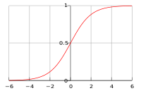 where the nonlinearity is the
logistic
function, shown at right
$$
s(z) = \frac{1}{1 + e^{-z}}.
$$
where the nonlinearity is the
logistic
function, shown at right
$$
s(z) = \frac{1}{1 + e^{-z}}.
$$
The effect of the logistic function is to "soft-clamp" the result of the linear model to 0 or 1, so that the influence of points far away from the decision boundary is small.
Gauss-Newton: Because the loss function is no longer quadratic, there is no longer a closed-form solution for the optimal parameters $\theta$ for this model. Instead, we will use an iterative method called Gauss-Newton.
The method starts by computing an initial estimate $\theta^{(0)}$ using simple linear regression, as above. (In this and all subsequent equations, parenthesized superscripts indicate values at different iterations. For example, $\theta^{(k)}$ refers to the value of $\theta$ after the $k$-th iteration.)
On each subsequent iteration, the method computes a "correction" to $\theta$ by solving a linear system. The linear system solved at each iteration comes from a first-order Taylor series expansion of the loss function around the current best estimate of $\theta$.
At each iteration, we compute the correction $\delta$ to be applied to $\theta$: $$ (J^TJ + \lambda\,n\,I)\,\delta^{(k)} = J^Tr^{(k-1)} $$ and apply it: $$ \theta^{(k)} = \theta^{(k-1)} + \delta^{(k)} $$
Here, $r^{(k-1)}$ is the vector of residuals after the $k-1$st iteration, defined as $$ r = \begin{pmatrix} z_1 - s(a + bx_{11} + cy_{12} + dy_{13} + \ldots) \\ z_2 - s(a + bx_{21} + cy_{22} + dy_{23} + \ldots) \\ \vdots \end{pmatrix} $$ and $J$ is the Jacobian (i.e., matrix of first derivatives) of $s$ applied to the linear model. As luck would have it, the derivative of $s$ has a particularly simple form: $$ \frac{ds(x)}{dx} = s(x) \, \bigl(1-s(x)\bigr) $$ and so the Jacobian is simple as well - it's just the data matrix $X$ multiplied by a diagonal "weight matrix" $W$: $$ J = W^{(k-1)} X, \quad \mathrm{where} \quad W_{ii} = s(x_i \cdot \theta^{(k-1)}) \bigl(1 - s(x_i \cdot \theta^{(k-1)}) \bigr) $$
Do this:
Download the starter code for this part.
It contains the following files:
Once you download the code, just run test_logistic in matlab. You will see four plots: ground-truth classification for both training and test data, and learned predictions on training and test. In addition, test_logistic will print out training and test accuracy. You should see it in the 85% range with the currently-implemented linear regression.
Read over the files and make sure you understand how they interact.
Implement logistic regression by modifying logistic_fit.m. Re-running test_logistic should result in much better classification performance.