Power
Problem Set 3: Map and Caml-Mathica
Quick Links:
- Part 1
- Part 2
- Compiling and Top-Levels for Part 2
- Problem 2.3
- Problem 2.4
- Problem 2.5
- Problem 2.6
- Problem 2.7 (optional)
Objectives
In this assignment, you will be given the opportunity to practice functional decomposition of complex problems into smaller, simpler ones. More specifically, you will look at functional decomposition of list processing problems in to subproblems that can be implemented by map, reduce, fold and filter functions. Functional programmers do this all the time in day-to-day programming tasks, but it is also the basis for programming parallel applications in frameworks like Hadoop or Google's Map-Reduce (it's no coincidence the names are the same!)
In addition, you will write your own language for symbolic differentiation using OCaml. This will illustrate just how easy it is to develop your own mini-language inside a functional language like OCaml using recursive data types and pattern matching.
Getting Started
Download the code here. Unzip and untar it:
$ tar xfz a3.tgzInside, you will see several files. The main ones you need to concern yourself with are:
mapreduce.mlwhich is a self-contained series of exercises involving higher order functions.expression.mlin which you will develop functions to perform symbolic differentiation of algebraic expressions.- Support code can be found in ast.ml and expressionLibrary.ml
- A
.merlinfile for Merlin to find your source code and additional files after you have compiled.
A few important things to remember before you start:
- This assignment must be done individually.
- Make sure that the functions you are asked to write have the correct names and the number and type of arguments specified in the assignment. Programs that do not compile will be subject to penalties on top of regular deductions.
- Style is naturally subjective, but the COS 326 style guide provides some good rules of thumb.
- As always, think first; write second; test and revise third. Aim for elegance.
- Compilation:
- make mapreduce compiles only Part 1.
- make expression compiles only Part 2.
- make and make all compile everything. (If you don't know why these two commands do the same thing, ask your preceptor.)
Part 1: Higher Order Functions (mapreduce.ml)
Map, filter and fold are functions that capture extremely common recursion patterns over lists. A good functional programmer uses these functions to construct solutions to interesting problems using very little code. In this part, you will get practice with higher-order functions by using map and fold to write a number of functions.
- map is implemented in OCaml by the function
List.map. - filter is implemented in OCaml by the function
List.filter. - fold is implemented in OCaml by the
function
List.fold_right. However, the standard OCaml library function has its arguments in an inconvenient order. Thus, we have provided you with the function "reduce" which computes identically to fold_right but takes arguments in a different order (discuss with your preceptor why this ordering is more useful).
All instructions for Part 1 can be found in mapreduce.ml, but as a reminder, the rec keyword and other explicit recursive solutions are prohibited for this part. You should be using higher-order functions to complete your tasks.
Part 2: A Language for Symbolic Differentiation (expression.ml)
In the Summer of 1958, John McCarthy (recipient of the Turing Award in 1971) made a major contribution to the field of programming languages. With the objective of writing a program that performed symbolic differentiation of algebraic expressions in a effective way, he noticed that some features that would have helped him to accomplish this task were absent in the programming languages of that time. This led him to the invention of LISP (published in Communications of the ACM in 1960) and other ideas, such as list processing (the name Lisp derives from "List Processing"), recursion, and garbage collection, which are essential to modern programming languages. Nowadays, symbolic differentiation of algebraic expressions is a task that can be conveniently accomplished on modern mathematical packages, such as Mathematica and Maple.
The objective of this part is to build a language that can differentiate and evaluate symbolically represented mathematical expressions that are functions of a single variable. Symbolic expressions consist of numbers, variables, and standard math functions (plus, minus, times, divide, sin, cos, etc).
Conceptual OverviewTo get you started, we have provided the datatype that defines the
abstract syntax tree for such expressions in ast.ml.
(* abstract syntax tree *)

(* Binary operators. *)
type binop = Add | Sub | Mul | Div | Pow ;;

(* Unary operators. *)
type unop = Sin | Cos | Ln | Neg ;;

type expression =
  | Num of float
  | Var
  | Binop of binop * expression * expression
  | Unop of unop * expression
;;
Var represents an occurrence of the single variable "x".
Unop(Ln, Var) represents the natural logarithm of x.
Neg is negation, and is denoted by the "~" symbol
("-" is only used for subtraction). The rest should be
clear what they refer to.
Mathematical expressions can be constructed using the
constructors in the above datatype definition. For example, the expression
"x^2 + sin(~x)" can be
represented as:
Binop(Add, Binop(Pow, Var, Num(2.0)), Unop(Sin, Unop(Neg, Var)))
This represents a tree where nodes are the type constructors and the children of each node are the specific operator to use and the arguments of that constructor. Such a tree is called an abstract syntax tree (or AST for short).
How to Compile and Test Part 2
The code you will be editing is in expression.ml. We have
used modules to keep this file clean and easy to navigate.
There are several ways to compile and test your code.
Easiest way: build-and-run
The easiest way to develop your code is in separate windows: one terminal to build your code and run the executable, and another window with your code.
- Edit your code until you are ready to test some part
- Type
make expressionin your shell, which will identify any compilation errors. - Run the compiled code with ./expression.d.byte, which will invoke any tests you have constructed.
- Evaluate the results of your tests and repeat.
More complicated (but maybe more useful?): toplevel
ocamlbuild does a great job of figuring out all the
dependencies for your program in order to give you a simple executable
to run. But it can complicate matters for running your program in the
toplevel interpreter.
Here are two list of steps to get part 2 running in the toplevel of your choice. First the stand-alone ocaml toplevel:
make- Start the toplevel with ocaml
- in the toplevel tell ocaml to look in the ocamlbuild _build directory with the command:
#directory "_build";; - in the toplevel tell ocaml to use the compiled expressionLibrary module with the command:
#load "expressionLibrary.cmo";; - now you can use your toplevel like normal, for instance loading your code with the command:
#use "expression.ml";;
make- emacs expression.ml
- merlin, if installed, should work immediately thanks to the .merlin file packaged with the assignment
- Start the toplevel (if you start it via an evaluation, ignore the "Unbound module Ast" error, we'll fix that in the next step)
- in the toplevel tell ocaml to look in the ocamlbuild _build directory with the command:
#directory "_build";; - in the toplevel tell ocaml to use the compiled expressionLibrary module with the command:
#load "expressionLibrary.cmo";; - now you can use your toplevel buffer like normal, for instance re-evaluating your entire with C-c C-b
# #load "expressionLibrary.cmo";;
Cannot find file expressionLibrary.cmo.
it probably means that you skipped step 1 (or have a bug) and thus have not successfully compiled your code prior to loading
expression.ml in to the toplevel environment.
Provided Infrastructure
We have provided some functions to
create and manipulate expression
values. checkexp is contained
in expression.ml. The others are contained in expressionLibrary.ml.
parse: translates a string in infix form (such as"x^2 + sin(~x)") into anexpression(treating "x" as the variable). Theparsefunction parses according to the standard order of operations - so"5+x*8"will be read as"5+(x*8)".to_string: prints expressions in a readable form, using infix notation. This function adds parentheses around every binary operation so that the output is completely unambiguous.make_exp: takes in a length l and returns a randomly generated expression of length at most 2l.rand_exp_str: takes in a length l and returns a string representation of length at most 2l.checkexp: takes in a string expression and an x value and prints the results of calling every function to be tested except find_zero.
Problem Instructions
Instructions for problems 2.1 and 2.2 are in expression.ml.
Problem 2.3: DerivativesNext, we want to develop a function that takes an expression
e as its argument and returns an expression
e' representing the derivative of the expression with
respect to x. This process is referred to as symbolic differentiation.
If you don't remember your calculus, here's the necessary crib sheet, some formulae for computing derivatives that you will use:
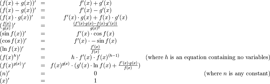
Note that there two cases provided for calculating the derivative of f(x) ^ g(x),
one for where g(x) = h does not contain any variables, and one for the general case.
The first is a special case of the second, but it is useful to treat them separately, because when
the first case applies, the second case produces unnecessarily complicated expressions.
Your task is to implement the derivative function.
The type of this function is expression -> expression.
The result of
your function must be correct, but need not be expressed in the simplest form.
Take advantage of this in order to keep the code in this part as short
as possible. You can implement this function in as little
as 20–30 lines of code.
To help you, we provide a function, checkexp,
which checks parts 2.1-2.3 for a given input. The portions of the function that
require your attention read failwith "Not implemented".
Do not attempt to run the function until you have replaced all of the
failwith expressions with valid code.
One application of the derivative of a function is to find zeros
of a function. One way to do so is Newton's
method. The function should take an expression, a guess
for the zero, a precision requirement, and a limit to the number of
iterations. If a guess g (to include the starting
guess) is sufficient to find a zero within the required precision,
it should immediately return Some g. Otherwise, so long
as the limit has not been reached, it should produce a new guess and
try again. It should return None if
no zero was found within the desired precision by the time the limit
was reached.
Your task is to implement the find_zero:expression ->
float -> float -> int -> float option function. Note that there are
cases where Newton's method will fail to produce a zero, such as for
the function x1/3. You are not
responsible for finding a zero in those cases,
but just for the correct implementation of Newton's method.
Note: If the expression that find_zero
is operating on is 'f(x)' and the precision is
epsilon, we are asking you to find a value
x such that |f(x)| < epsilon. That is, the
value that the expression evaluates to at x is "within
epsilon" of 0.
We are not requiring you to find an x such that |x -
x0| < epsilon for some x0 for
which f(x0) = 0.
The function you wrote above allows you to find the zero (or a zero) of most functions that can be represented with our AST. This makes it quite powerful. However, in addition to numeric solving like this, Mathematica and many similar programs can perform symbolic algebra. These programs can solve equations using techniques similar to those you learned in middle and high school (as well as more advanced techniques for more complex equations) to get exact, rather than approximate answers.
Performing symbolic manipulation on complex expressions is quite difficult, and we do not expect you to do it. However, there is one type of expression for which this is not so difficult. These are polynomial expressions that can be simplified to the form ax + b. You likely learned how to solve equations of the form ax + b=0 years ago, and can apply the same skills in writing a program to solve these.
More specifically, for the purposes of this question,
a
- contains only Add, Sub, Mul, and Neg operators (nested arbitrarily)
- can be simplified to the form ax + b.
Your task is to write the function find_zero_exact,
which will exactly find the zero of those degree-one expressions that
do have zeros. More specifically, for degree-one expressions that do
have zeros your function should return Some of an
expression that
- contains no variables
- evaluates to the zero of the given expression and
- is exact.
None.
Note: degree one expressions need not be as simple as ax + b. Something like 5x - 3 + 2(x - 8) is also a degree-one expression since it can be turned into ax + b by distributing and simplifying. Likewise x*x - x*x + x can be simplified to x since the quadratic expression cancels.
You need not return the simplest expression. For example,
find_zero_exact (parse "3*x-1") might return Binop
(Div, Num 1., Num 3.) or Unop(Neg, Binop (Div, Num -1.,
Num 3.)). You may also assume idealized floating point
arithmetic (+., -., *. never overflow and result in exact values) and
return Num result where result is the answer
you get when dividing -1. by 3.
You will need to think about how to handle various forms of degree one expressions. You will also need to think about how to determine whether an expression is degree one in the first place. You should aim for a very general solution, because handling individual cases with clever logic is intractable beyond very basic examples! We suggest converting each subexpression into some kind of standard form, and then manipulating those standard forms.
How you handle these operations must be, at the core, symbolic
manipulation instead of a series of evaluation steps. An example of
the latter would be first confirming degree-one by evaluating the
second derivative and comparing with 0, and then evaluating the
function at 0 and 1 to determine the two coefficients of the
closed-form solution x = -a0/a1. Do
not do this, as computational solutions like this will receive no credit.
Finally, we ask you to do a better job of expressing expressions as strings. Specifically, write a function, to_string_smart that prints expressions in an even more readable form, only adding parentheses when there may be ambiguity.
Rules concerning parenthesis placement:
- Always put parentheses around the argument to a unary operation. eg: sin(cos(x)) or ~(3.0).
- Never put two sets of parentheses in a row. eg: never like this: sin((x + y)). Otherwise:
- If a child operator's precedence is less than its parent operator's precedence, then no parentheses are needed around the child operation. eg: x + 3.0*x or (x + 3.0) * x
- If a child operator is the same operator as its parent, and that operator is associative, then no parentheses are needed around the child operation. eg: 2.0 + 3.0 + 4.0
Precedence of operators:
- Add, Sub = 3
- Mul, Div = 2
- Pow = 1
- All unary operators = 0
Another example of the difference between to_string and to_string_smart:
let e = Binop(Add,Binop(Pow,Var,Num 2.0),Unop(Sin,Binop(Div,Var,Num 5.0)))
  to_string(e) = "((x^2.)+(sin((x/5.))))"
  to_string_smart(e) = "x^2.+sin(x/5.)"
Optional Problem 2.7: The amazing effectiveness of Newton's method.
Newton's method often converges really fast!
Consider using it to calculate sqrt(N):
let f N x = x^2 - N
To find sqrt(N), just find a zero of the function (f N).
If you want K bits of precision, how many iterations of Newton's method do you have to run? Let newton(f N,N,i) be the result of running i iterations of Newton's method on that function (f N) with starting point N. Now calculate E(i) = -lg(abs(newton(f N, N, i) - sqrt(N))), where lg is the binary logarithm. That tells you how many bits of accuracy you have after i iterations. How does E grow as a function of i? How many iterations do you need to calculate to 56 bits of accuracy, which the length of the mantissa of double-precision floating point? That's how your computer's sqrt function actually works, by the way.
How many points is this "optional" thing worth?Perhaps none at all. Some things you do because they are intellectually interesting. If it's not interesting, or if you're pressed for time, leave it out.
Handin Instructions and Grading Information
This problem set is to be done individually.
You must hand in these files to dropbox (see link on assignment page):
-
mapreduce.ml -
expression.ml
Final Warning: Before you submit, be sure to
compile your code one last time with make and then to
test that none of your tests fail by running the mapreduce and
expression executables produced by using make. You should
also make sure that the "check all submitted files" button on dropbox
does not report any compilation errors nor abort with an
exception.
Assignments that do not compile will be treated harshly. It is
much better to turn in an assignment that compiles but is incomplete
than to turn in an assignment that does not compile. If you do not
have a compiling version of a function, please comment out all your
code for that function rather than reverting to the failwith
"Not implemented" line; this way your files will still compile
and will not disrupt the automatic grader. Document in a comment
anything you tried or any problems you had with a particular portion
of the assignment.
There are 30 total points in this assignment, broken down as 5 for problem 1.1, 10 for problem 1.2, and 15 for problem 2. Further subdivisions are as follows:
- Each subproblem 1.1.a-1.1.e: 1
- Each subproblem 1.2.a-1.2.e: 2
- Problem 2.1: 1
- Problem 2.2: 2
- Problem 2.3: 3
- Problem 2.4: 2
- Problem 2.5: 5
- Problem 2.6: 2