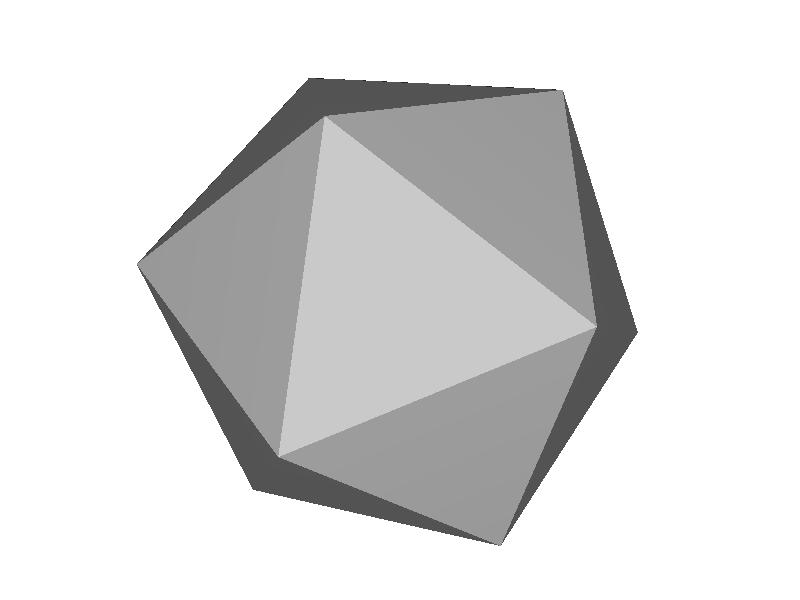
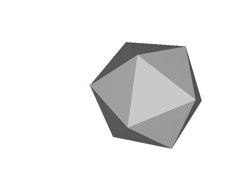
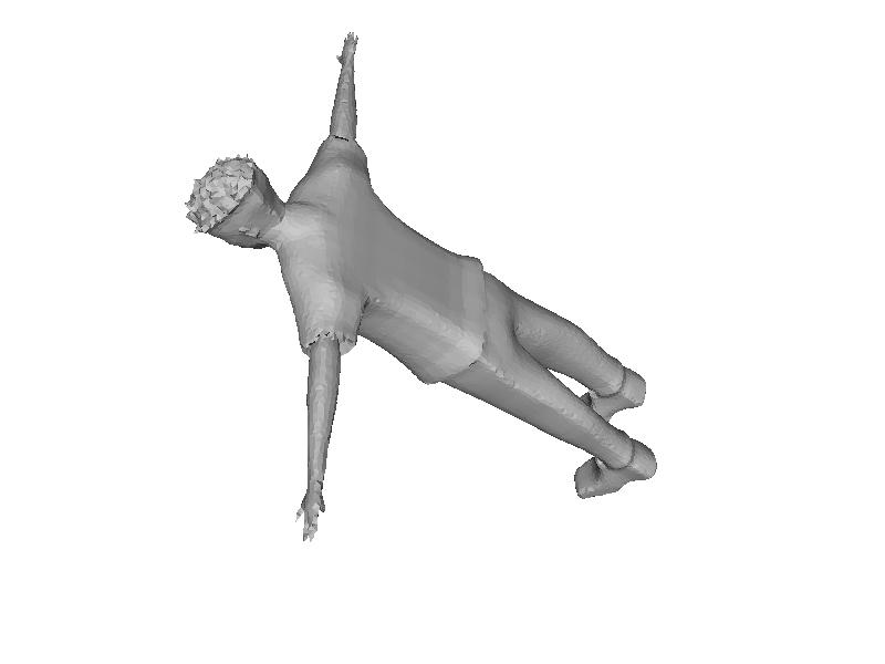
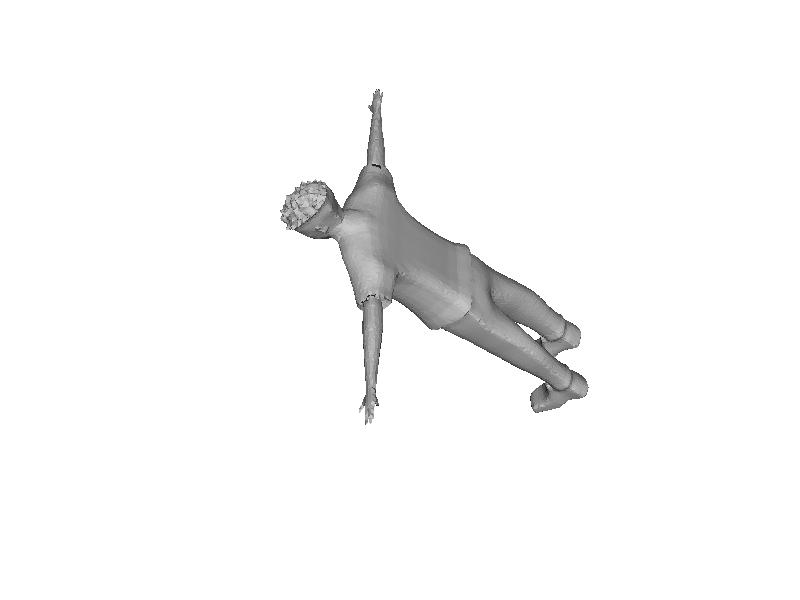
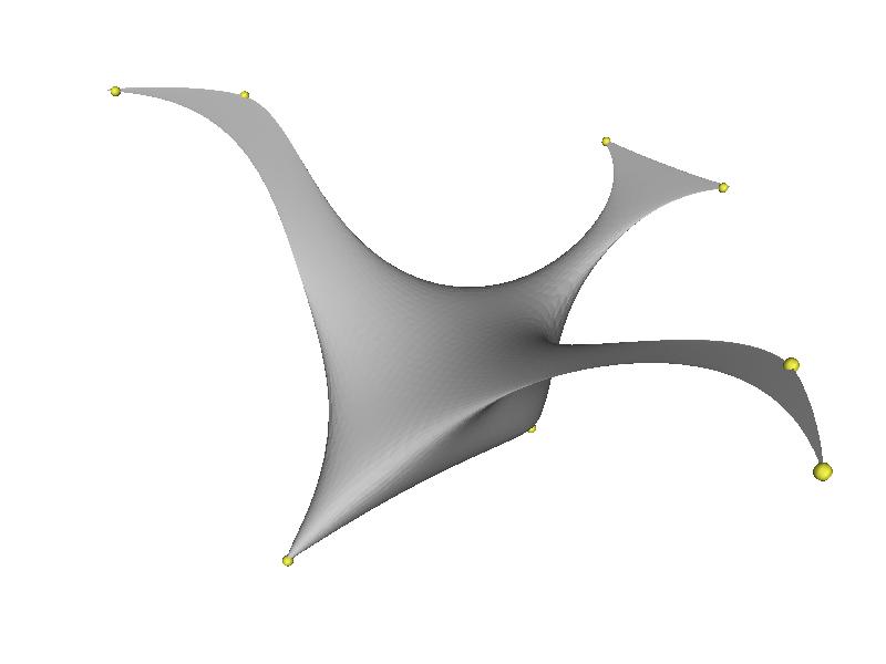
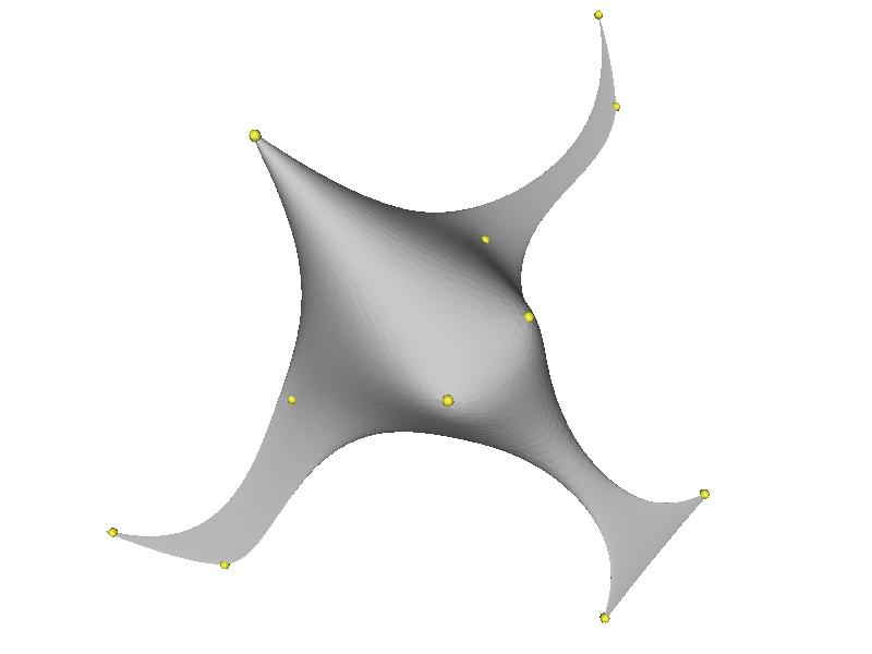
I use CSparse to solve the linear problem in mesh reconstruction. After anchoring the position of a vertex (v(0) = (0, 0, 0)), the original mesh is reconstructed, yet translated to a new position. Results are shown in Figure 1 and Figure 2.
Figure 1a. Original(ico)
Figure 1b. Reconstructed(ico)
Figure 2a. Original(boy)
Figure 2b. Reconstructed(boy)
Mesh Deformation
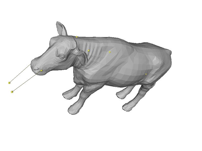
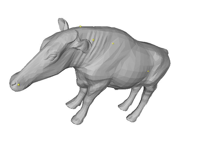
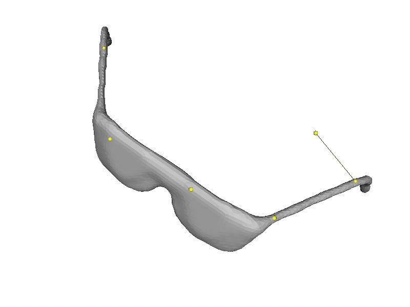
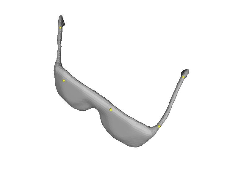
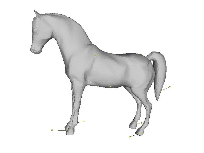
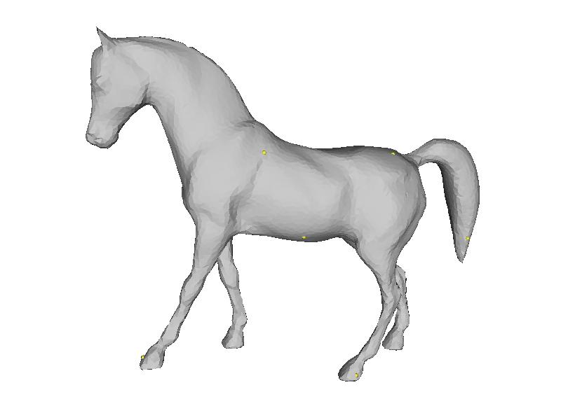
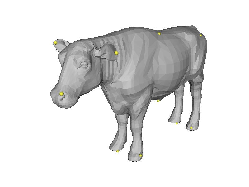
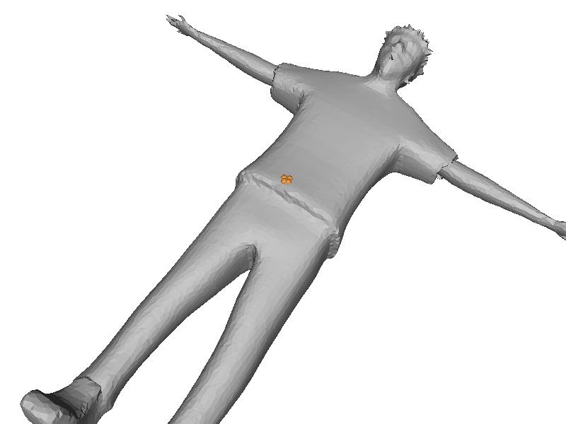
By adding new entries into laplacian matrix, we put constraints on the positions of anchored vertices. We select the value of the maximum entry that appears in the diagonal of laplacian matrix as the weight of newly-added entries. Results are shown in Figure 3, 4, 5.
Figure 3a. Anchored Vertices(cow)
Figure 3b. Result(cow)
Figure 4a. Anchored Vertices(glasses)
Figure 4b. Result(glasses)
Figure 5a. Anchored Vertices(horse)
Figure 5b. Result(horse)
Parameterization
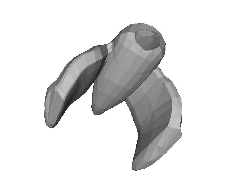
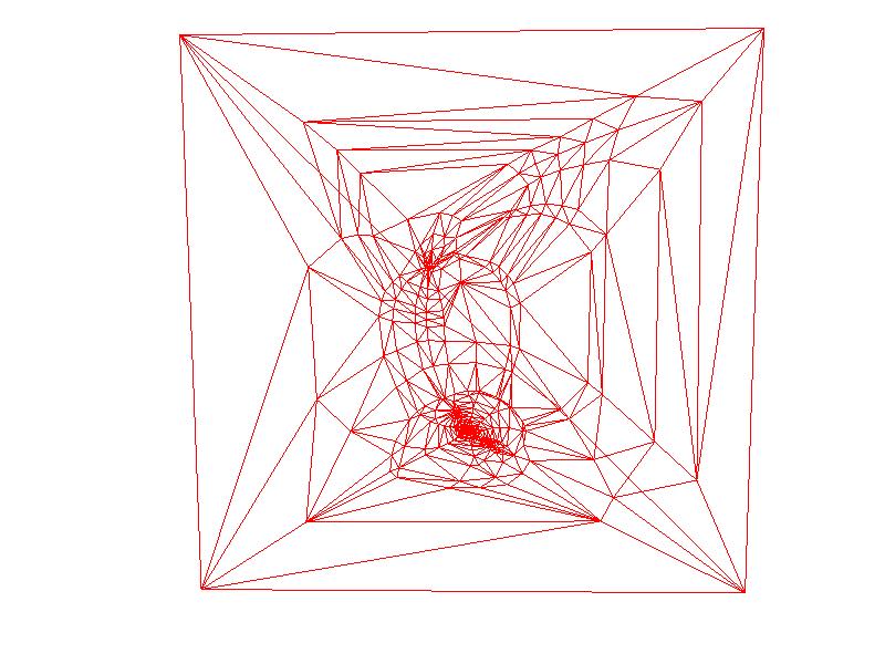
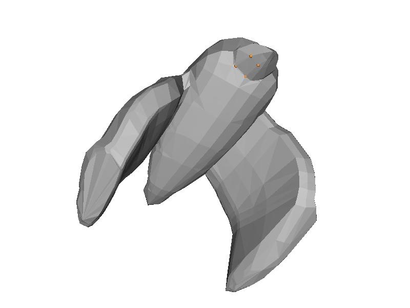
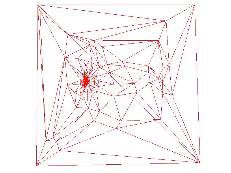
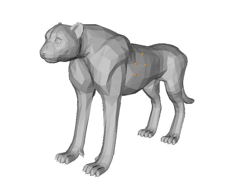
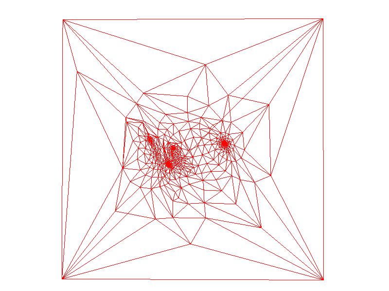
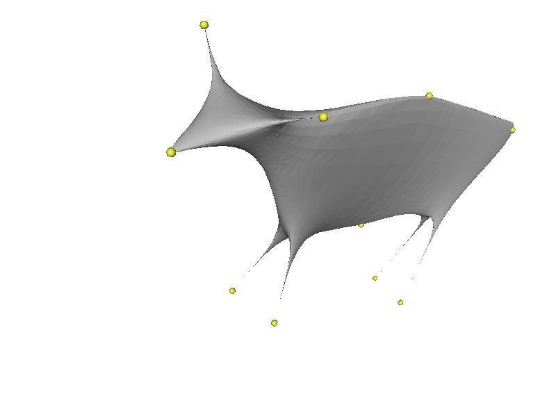
After picking 4 vertices on the meshes (forming two neighboring triangles), I replace the corresponding 4 rows in the laplacian matrix, so that I put constraints on the positions of the four vertices instead of their sigma coordinates. If new entries are added into the matrix insteading of replacing, the result will be problematic, since the sigma coordinates on the corners tend to pull vertices out of the square. Results are shown in Figure 6, 7, 8.
Figure 6a. Corner Vertices(bird)
Figure 6b. Parameterization(bird)
Figure 7a. Corner Vertices(bird)
Figure 7b. Parameterization(bird)
Figure 8a. Corner Vertices(cheetah)
Figure 8b. Parameterization(cheetah)
Membrane Surface
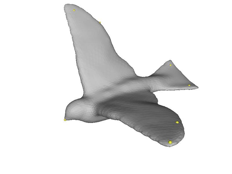
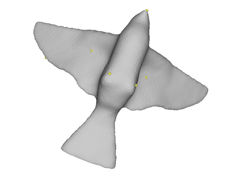
Fixed some vertices, and keep laplacian coordinates to be 0 on other vertices. Results are shown in Figure 9, 10.
Figure 9a. Anchored Vertices(cow)
Figure 9b. Membrane(cow)
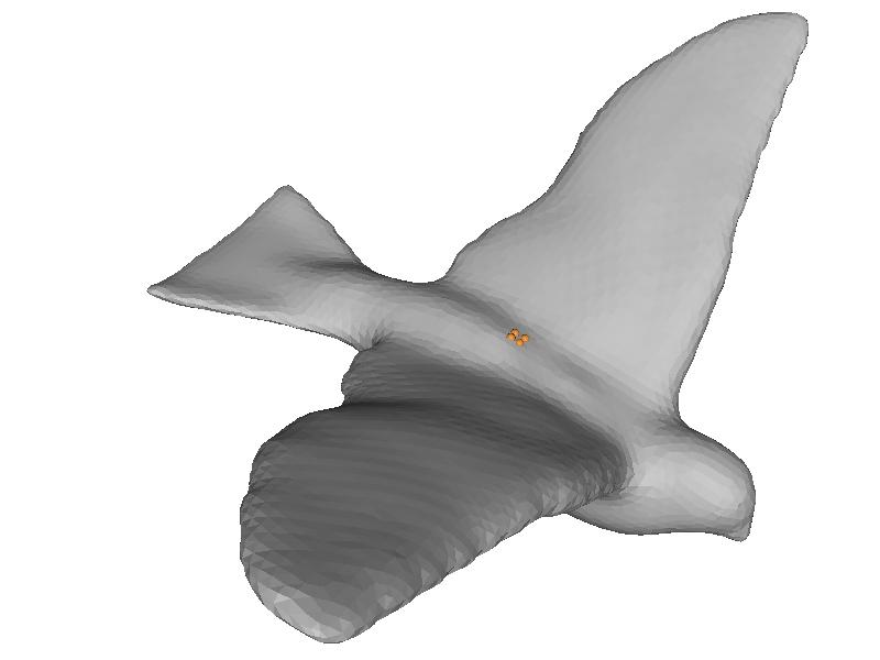
Figure 10a. Anchored Vertices(pigeon)
Figure 10b. Anchored Vertices(pigeon)
Figure 10c. Membrane(pigeon)
Figure 10d. Membrane(pigeon)
Function Interpolation
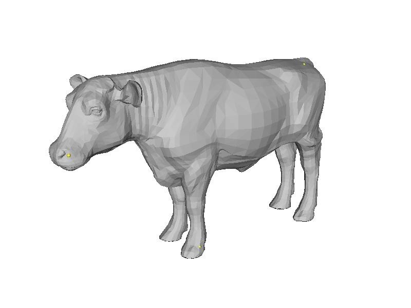
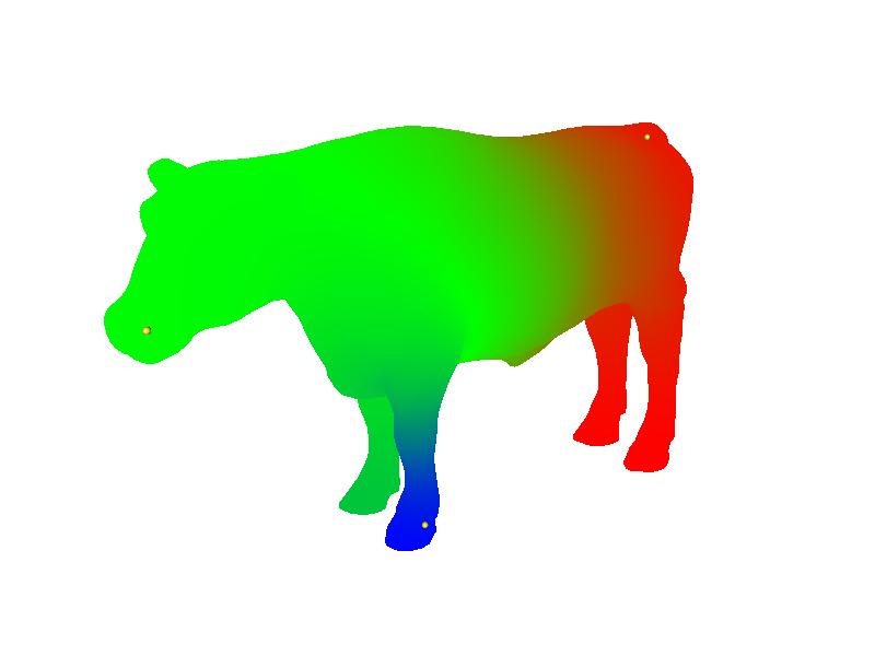
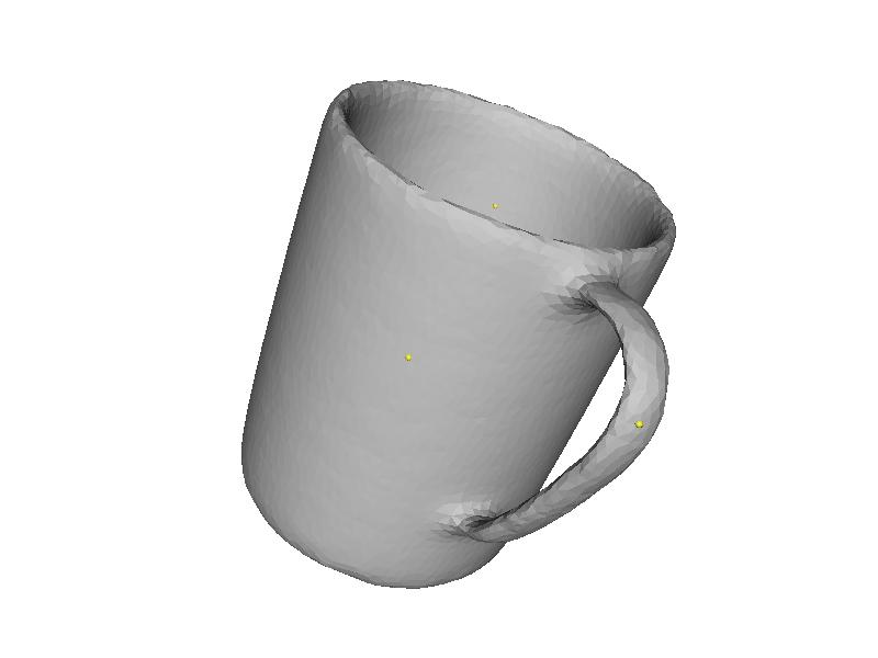
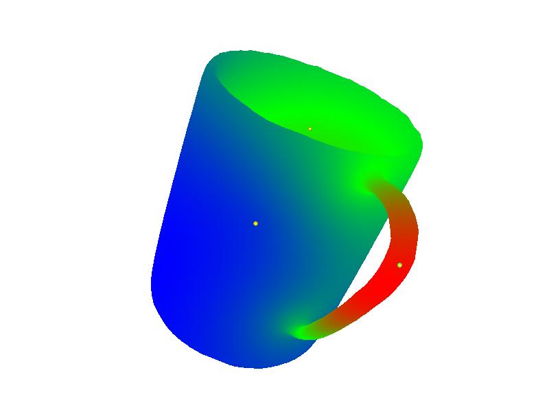
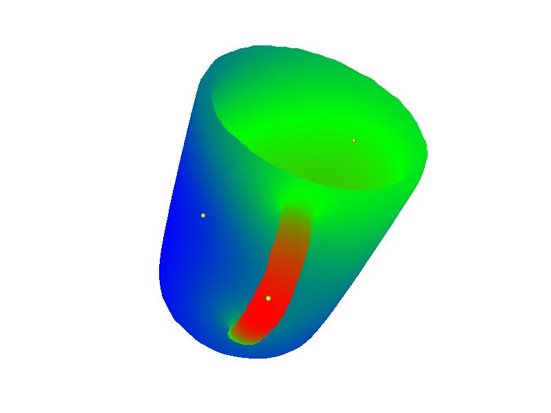
Take the vertices with given value as constraints, and set all sigma coordinates as 0 (make the value on a vertex tend to be the average of the values on its neighbors). In the following examples, I pick 3 vertices on each mesh, and set the values on the three vertices to be 100, 200, 300. Results are shown in Figure 11, 12, 13.
Figure 11a. Picked Vertices(cow)
Figure 11b. Value Visualization(cow)
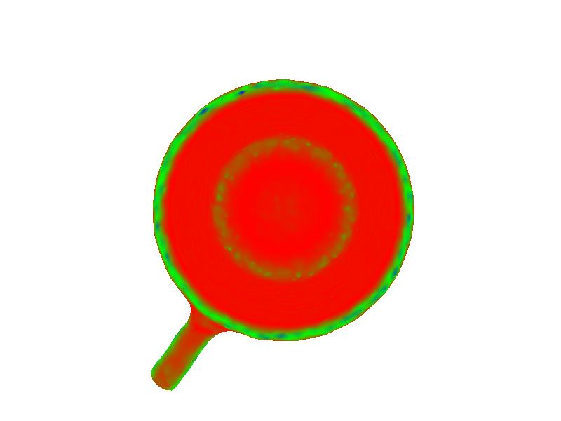
Figure 12a. Picked Vertices(cup)
Figure 12b. Value Visualization(cup)
Figure 12c. Value Visualization, another side(cup)
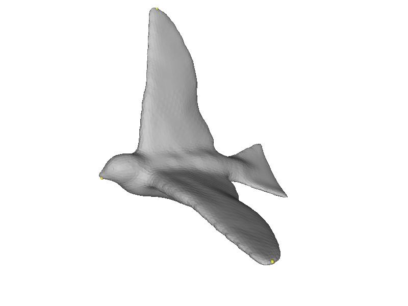
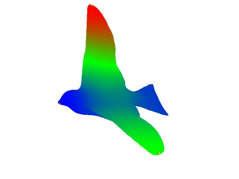
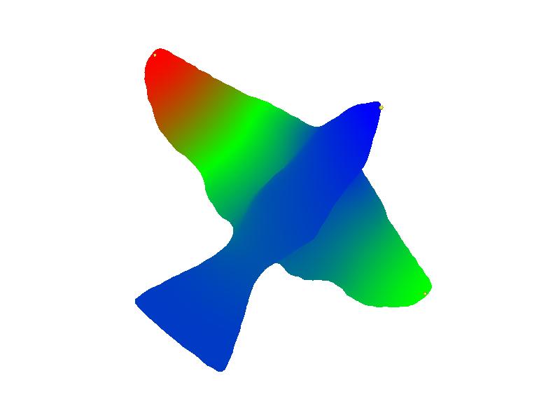
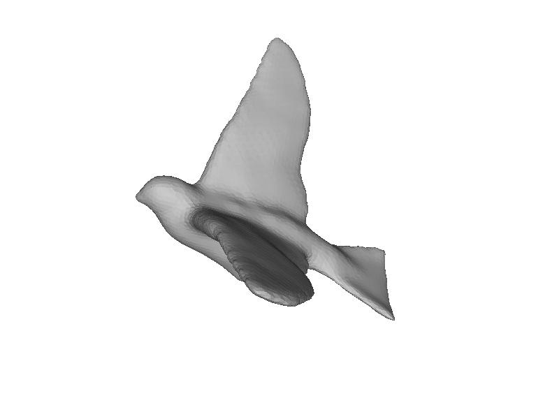
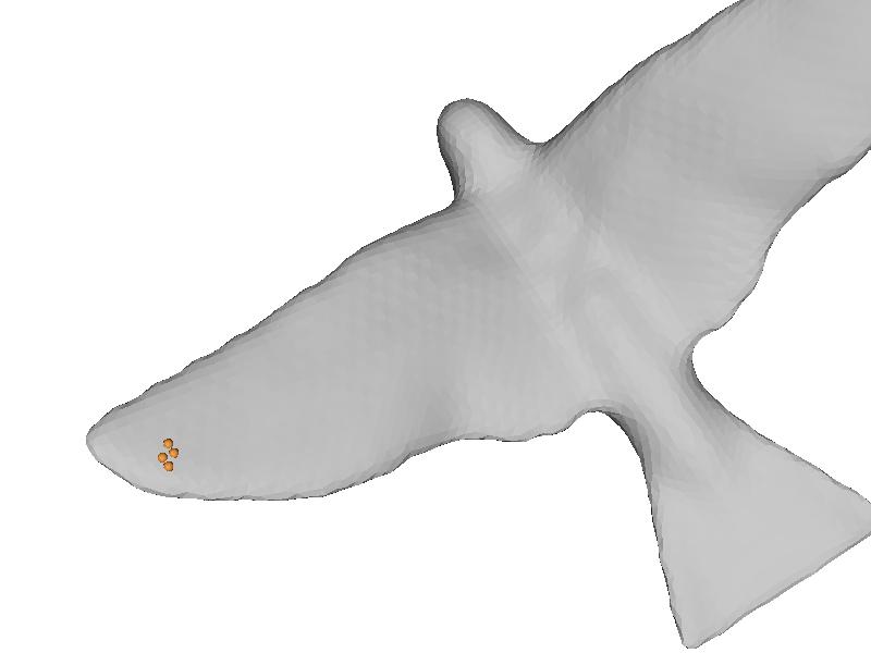
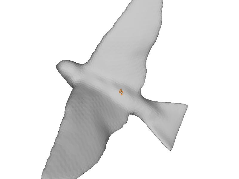
Figure 13a. Picked Vertices(pigeon)
Figure 13b. Value Visualization(pigeon)
Figure 13c. Value Visualization, another side(pigeon)
Mean Curvature
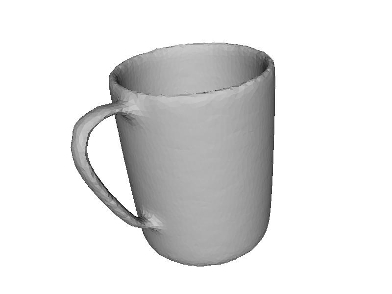
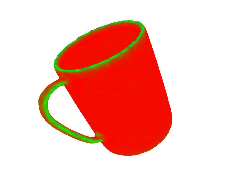
Use cotangent formula to mimic mean curvature. Note that this method is problematic when triangle is obtuse, therefore I try my best to find good meshes for this application, where most triangles are normal. Results are shown in Figure 14, 15, 16.
Figure 14a. Input(cup)
Figure 14b. Curvature Visualization(cup)
Figure 14c. Curvature Visualization, another side(cup)
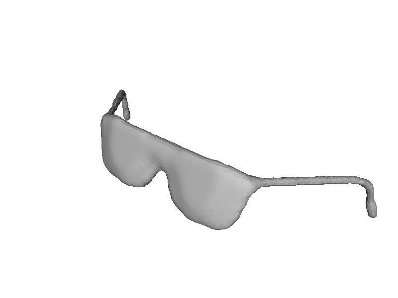
Figure 15a. Input(glasses)
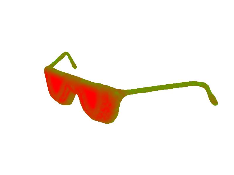
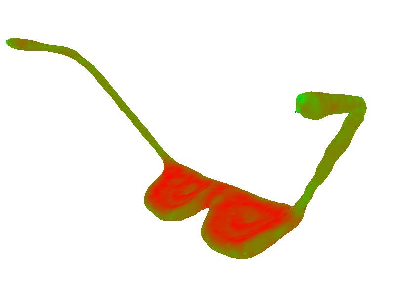
Figure 15b. Curvature Visualization(glasses)
Figure 15c. Curvature Visualization, another side(glasses)
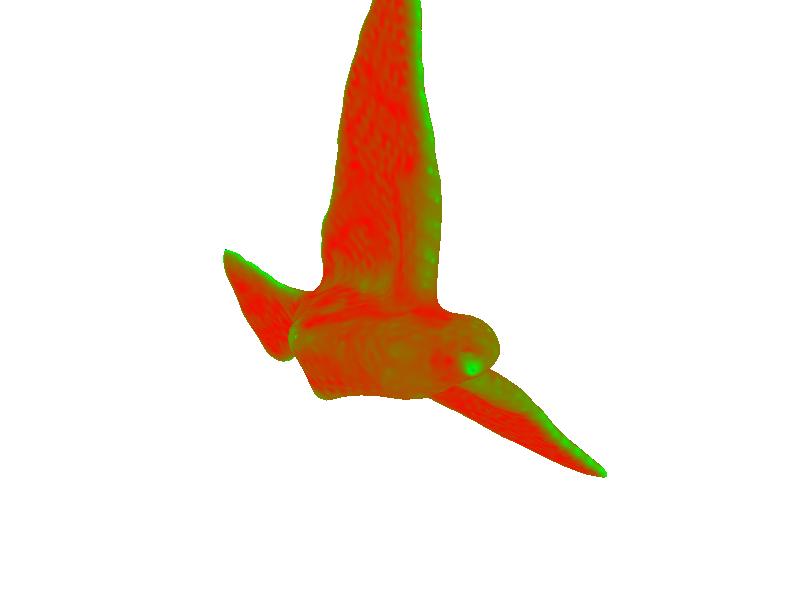
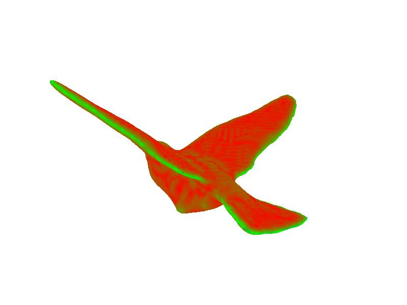
Figure 16a. Input(pigeon)
Figure 16b. Curvature Visualization(pigeon)
Figure 16c. Curvature Visualization, another side(pigeon)
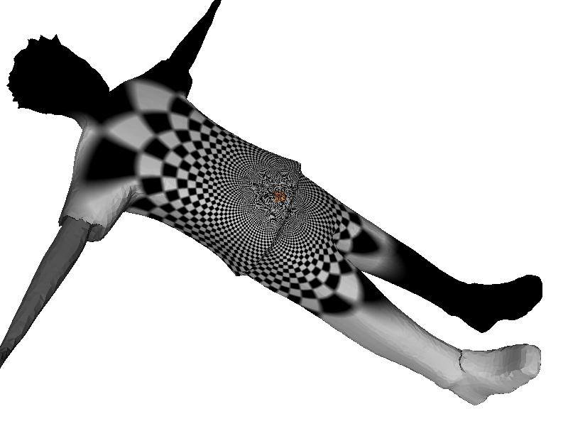
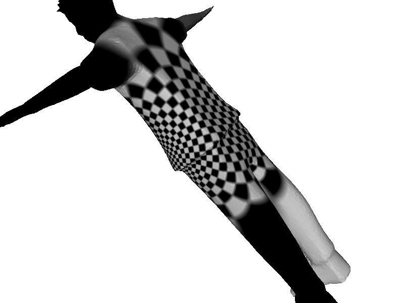
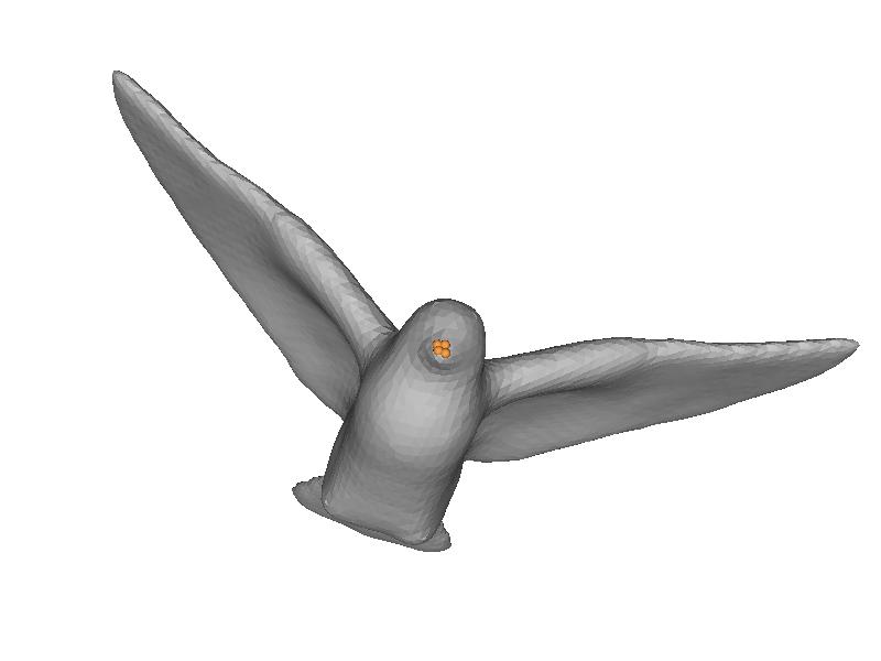
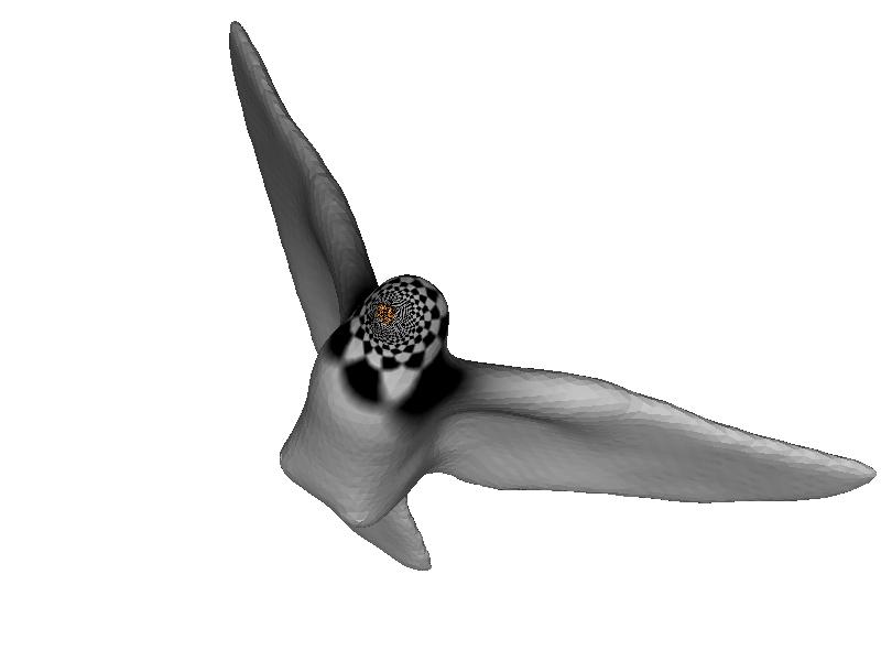
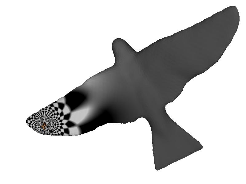
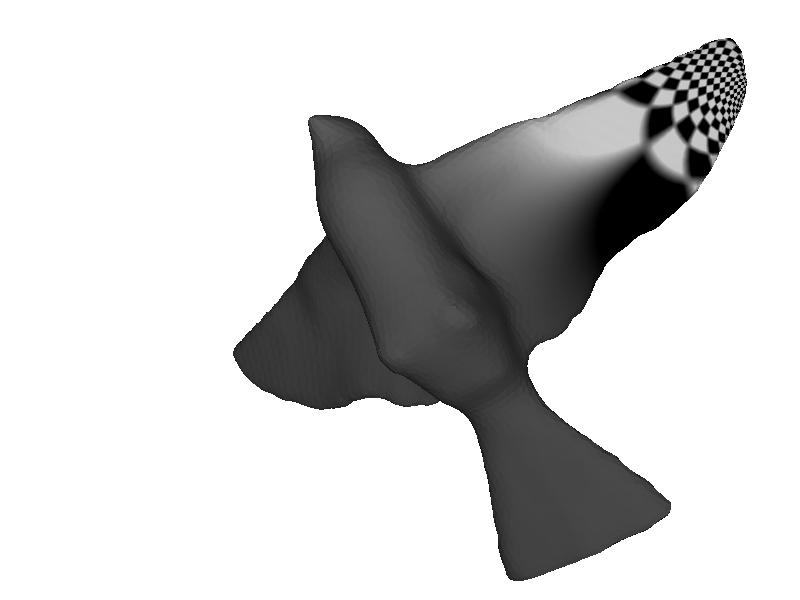
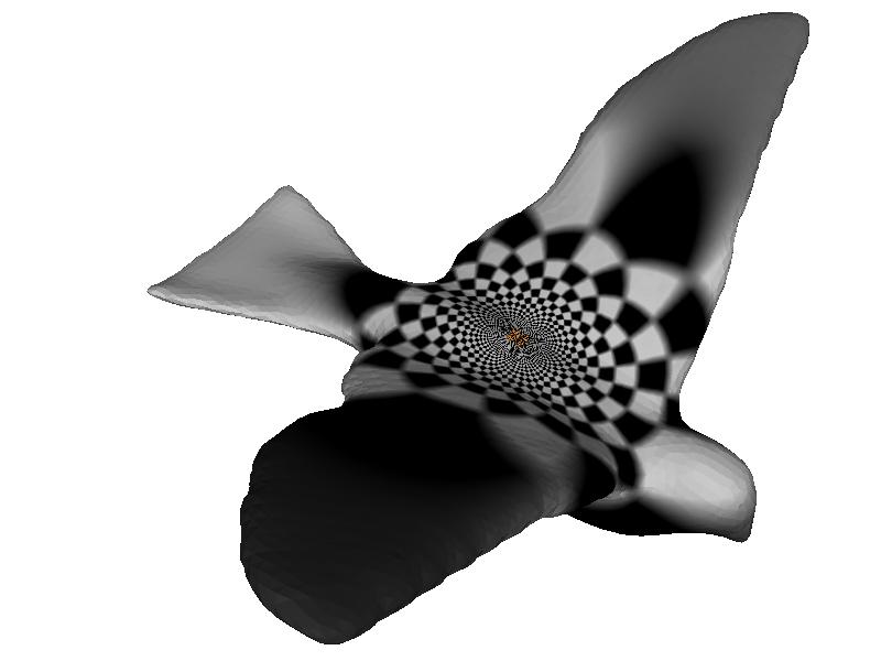
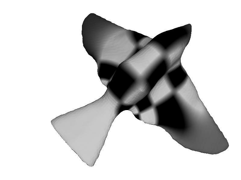
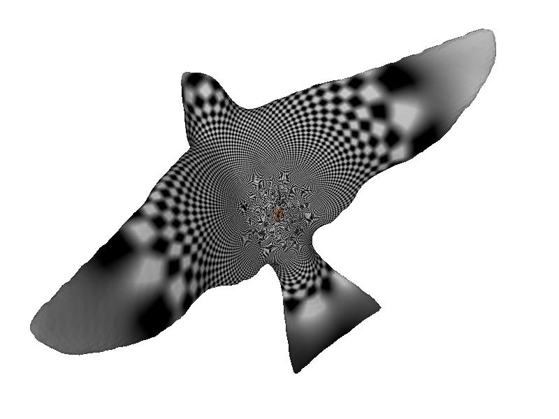
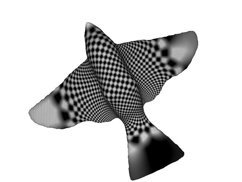
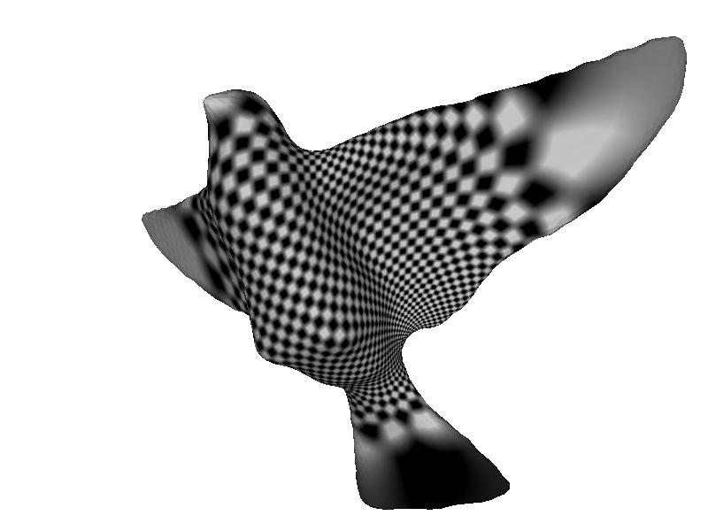
Texture Mapping
Uae the result of parameterization, to map checker boarder onto the mesh. Unfortunately, since parameterization given above is not an ideal one, it causes great distortion around the selected 'corner vertices'. The size of boxes vary greatly. Results are shown in Figure 16, 17, 18, 19, 20.