COS 323 - Computing for the Physical and Social Sciences

Fall 2012

Assignment 2: Logistic Regression

In this assignment, you will implement nonlinear least squares fitting using Gauss-Newton iteration. You will be fitting to the logistic model, which (under certain assumptions) predicts the probability of occurrence of some event as a function of the values of some explanatory variables.

1. Derivation

The logistic model is a generalized linear model, meaning that the function consists of a single nonlinearity applied to a linear combination of the variables: $$ p(x) = g(a + b x_1 + c x_2 + \cdots) $$

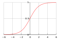
where the nonlinearity is the logistic function, shown at right $$ g(z) = \frac{1}{1 + e^{-z}}. $$

In this case, the explanatory variables are $x_1, x_2, \ldots$, and any given setting of them gives rise to a probability. Fitting the logistic model to data consists of estimating the coefficients $a, b, c, \ldots$ using least squares: $$ \arg\min \; \sum_{i=1}^{n} \bigl(y_i - g(a + b x_{i1} + c x_{i2} + \cdots)\bigr)^2 . $$ For the double-subscripted variables $x_{ij}$, the first subscript refers to the data point and the second refers to which explanatory variable it is. Since for each data point the event actually did or did not occur, the $y_i$ will each be 0 or 1. Note that the above includes a constant term, which was not included in the lecture notes.

You will be using Gauss-Newton iteration to perform the fit - see the motivation behind this in slides 8-18 of Lecture 8. Briefly, you will compute successively better estimates of the parameters via the iteration $$ \begin{pmatrix} a \\ b \\ c \\ \vdots \end{pmatrix}^{\!\!(k+1)} = \begin{pmatrix} a \\ b \\ c \\ \vdots \end{pmatrix}^{\!\!(k)} + \delta^{(k)}, \quad \mathrm{where} \quad J^\mathrm{T} J \, \delta = J^\mathrm{T} r. $$

The matrix $J$ is a Jacobian: the columns correspond to partial derivatives of $p(x)$ with respect to $a, b, c, \ldots$, and each row corresponds to a different data point. The vector $r$ is the residual: each row is $y_i - g(a + b x_{i1} + c x_{i2} + \cdots)$ for a different data point. (The parenthesized superscripts $(k)$ and $(k+1)$ are the values at different iterations.)

To do: Derive the expression for each row in the Jacobian. Remember to use the chain rule for differentiation. Hint: the derivative of the logistic function $g(z)$ may be written as just $g(z)\,(1-g(z))$, which should simplify your expressions (and hence your code).

2. Implementation

Implement a Matlab function, or collection of functions, that performs the following:

1. Takes as input a matrix in which each row contains $y_i$ (zero or one) and some number of $x_{ij}$.
2. Carries out a Gauss-Newton iteration using the derivations you did above. Use SVD to aid in solving the linear system.

   Hint #1: Use the [U,W,V] = svd(A,0); syntax.
   Hint #2: You should never need to compute $J^\mathrm{T} J$ explicitly.

3. Terminates the iteration at a point of your choosing. Justify your termination condition in the writeup.
4. Returns the best-fit parameters $a,b,c,\ldots$ as well as the condition number of $J^\mathrm{T} J$ from the last iteration.

3. Evaluation

Test your implementation on the file gradschool.csv, which you can load with the command

load -ascii gradschool.csv

• The first column is 1 if accepted, 0 if not accepted.
• The second column is GRE score.
• The third column is GPA.
• The fourth column is prestige of undergrad institution.

Try running the regression on several different subsets of the data. What can you say about the stability with which each parameter is recovered? 

Submitting

This assignment is due Tuesday, October 23, 2012 at 11:59 PM. Please see the course policies regarding assignment submission, late assignments, and collaboration.

Please submit:

• Your code from Section 2, in one or more well-commented .m files.
• Submit an assignment writeup in a plain-text or PDF file, containing:
• A description of your code (minimally: which files contain solutions for Sections 2 and 3, and a brief description of how they work).
  
• Your derivation of the Jacobian for Section 1.
• Justification of your termination condition for Section 2.
• Discussion of stability for Section 3.
  
• Any additional notes or comments you feel are necessary for us to understand your assignment and grade it fairly and easily.
  

The Dropbox link to submit your assignment is here.